Usage

To use LaTeXiPy in a project:

import latexipy as lp

Set up for LaTeX with:

lp.latexify()

And make your figures with:

with lp.figure('filename'):
    draw_the_plot()

Import from LaTeX with:

\usepackage{pgf}
\input{filename.pgf}

Example files

From the latexipy Github repository.

• Python
• Latex
• PDF

Minimum Working Example

sincos_plotter.py

import numpy as np
import matplotlib.pyplot as plt

import latexipy as lp

lp.latexify()

with lp.figure('sincos'):
    x = np.linspace(-np.pi, np.pi)
    y_sin = np.sin(x)
    y_cos = np.cos(x)
    plt.plot(x, y_sin, label='sine')
    plt.plot(x, y_cos, label='cosine')
    plt.title('Sine and cosine')
    plt.xlabel(r'$\theta$')
    plt.ylabel('Value')
    plt.legend()

sincos_report.tex

\documentclass{article}

\usepackage{pgf}

\begin{document}
  \begin{figure}[h]
    \centering
    \input{img/filename.pgf}
    \caption[LOF caption]{Regular caption.}
    \label{fig:pgf_example}
  \end{figure}
\end{document}

Plotting

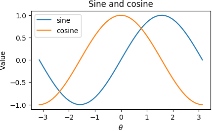
Without LaTeX

If you are not making your plots for LaTeX, Matplotlib’s defaults are used. The typeface is sans-serif, and the font, a bit large. The default arguments save a PGF and PNG file in the img/ directory.

with lp.figure('sincos'):
    plot_sin_and_cos()

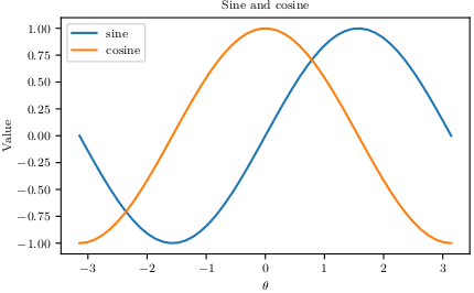
With LaTeX

If you are building for LaTeX, just lp.latexify()!

lp.latexify()

with lp.figure('sincos'):
    plot_sin_and_cos()

Using custom parameters

By default, lp.latexify() uses lp.PARAMS, which has the following values:

_latexipy.py

FONT_SIZE = 8

PARAMS = {
    'pgf.texsystem': 'xelatex',  # pdflatex, xelatex, lualatex
    'text.usetex': True,
    'font.family': 'serif',
    'font.serif': [],
    'font.sans-serif': [],
    'font.monospace': [],
    'pgf.preamble': [
      r'\usepackage[utf8x]{inputenc}',
      r'\usepackage[T1]{fontenc}',
      ],
    'font.size': FONT_SIZE,
    'axes.labelsize': FONT_SIZE,
    'axes.titlesize': FONT_SIZE,
    'legend.fontsize': FONT_SIZE,
    'xtick.labelsize': FONT_SIZE,
    'ytick.labelsize': FONT_SIZE,
}

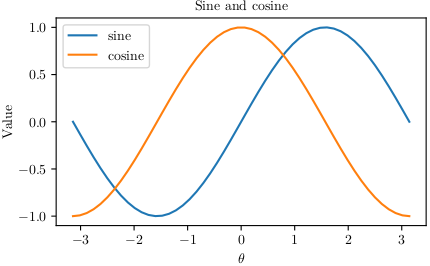
Passing a different dictionary to lp.latexify() causes these changes to be permanent in the rest of the code. For example, to increase the font size throughout:

examples.py

    font_size = 10
    params = lp.PARAMS.copy()
    params.update({param: font_size
                   for param in params
                   if 'size' in param})
    lp.latexify(params)

    with figure('sincos_big_font_permanent'):
        plot_sin_and_cos()

You can call lp.latexify() multiple times throughout your code, but if you want to change the setting only for a few figures, the recommended approach is to use lp.temp_params(). This automatically reverts to the previous settings after saving (or attempting to save) the plot.

examples.py

    font_size = 10
    with lp.temp_params(font_size=font_size):
        with figure('sincos_big_font_temp'):
            plot_sin_and_cos()

Either way, the font size would have increased uniformly from 8 to 10 pt.

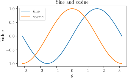
Note that lp.temp_params() can also take a custom dictionary which can do more fine-grained tuning of fonts.

examples.py

    with lp.temp_params(font_size=10, params_dict={
        'axes.labelsize': 12,
        'axes.titlesize': 12,
        }):
        with lp.figure('sincos_big_label_title'):
            plot_sin_and_cos()

Reverting

To revert all changes made with lp.latexify() and other commands, just run lp.revert().

Avoiding repetition

If you keep passing the same arguments to lp.figure() (for example, an output directory, a set of filetypes, or a certain size), you can save it for reuse by using functools.partial(). After that, you can use it just like lp.figure(). Note that you would not be able to redifine an argument that you had previously applied.

figure = partial(lp.figure, directory=DIRECTORY)

with figure('sincos_partial'):
    plot_sin_and_cos()

where DIRECTORY is the default output directory. This pattern was used extensively in the Python file from the examples directory.

Using in LaTeX

To include a PGF file in your LaTeX document, make sure that the pgf package is loaded in the preamble.

\usepackage{pgf}

After that, you can include it in the correct location with:

\input{<filename>.pgf}

A minimum working example of an image within a figure is shown below.

\documentclass{article}

\usepackage{pgf}

\begin{document}
  \begin{figure}[h]
    \centering
    \input{img/filename.pgf}
    \caption[LOF caption]{Regular caption.}
    \label{fig:pgf_example}
  \end{figure}
\end{document}

Note that figures using additional raster images can only be included by \input{} if they are in the same directory as the main LaTeX file. To load figures from other directories, you can use the import package instead.

\usepackage{import}
\import{<path to file>}{<filename>.pgf}

A minimum working example of that scenario is shown below.

\documentclass{article}

\usepackage{import}
\usepackage{pgf}

\begin{document}
  \begin{figure}[h]
    \centering
    \import{/path/to/file/}{filename.pgf}  % Note trailing slash.
    \caption[LOF caption]{Regular caption.}
    \label{fig:pgf_example}
  \end{figure}
\end{document}